API User’s Guide
Data Files
When performing a measurement with SnowMicroPen, the device writes the data
onto its SD card in a binary file with a pnt extension. (Example:
S13M0067.pnt). For each measurment process, a new pnt file is written.
Each pnt file consists of a header with meta information followed by the actual
data, the force samples.
Note
The snowmicropyn package never ever writes into a pnt file. Good to know your precious raw data is always save.
Corresponding ini files
However, when using functionality of this package, an additional storage to save
other data is required. This storage is an ini file, named like the pnt
file (Example from section before: S13M0067.ini).
First steps
The core class of the API is the snowmicropyn.Profile class. It
represents a profile loaded from a pnt file. By using its static load method,
you can load a profile:
import snowmicropyn
p = snowmicropyn.Profile.load('./S13M0067.pnt')
In the load call, there’s also a check for a corresponding ini file, in this
case for the S13M0067.ini.
Logging snowmicropyn’s Version and Git Hash
As a scientist, you may interested to keep a log so you can reproduce what you calculated with what version of snowmicropyn. The package contains a version string and a git hash identifier.
To access the packages version string, you do:
import snowmicropyn
v = snowmicropyn.__version__
To access the git hash string of this release, you do:
import snowmicropyn
gh = snowmicropyn.githash()
When exporting data using this module, the created CSV files also will contain a comment as first line with version string and git hash to identify which version of snowmicropyn was used to create the file.
Warning
However, this is no mechanism to protect a file from later alternation. It’s just some basic information which maybe will be useful to you.
Examples
Some examples will help you to get an overview of snowmicropyn’s features.
Hint
To get the code mentioned in this guide, Download the source code of
snowmicropyn. You’ll find the examples in the subfolder examples
and even some pnt files to play around with in the folder
examples/profiles.
Explore properties
In our first example, we load a profile and explore its properties. We set some
markers and finally call the snowmicropyn.Profile.save() so the markers
get save in a ini file so we don’t loose them.
import logging
import sys

import snowmicropyn

# Enable logging to stdout to see what's going on under the hood
logging.basicConfig(level=logging.DEBUG, stream=sys.stdout)

print(snowmicropyn.__version__)
print(snowmicropyn.githash())

p = snowmicropyn.Profile.load('profiles/S37M0876.pnt')

print('Timestamp: {}'.format(p.timestamp))
print('SMP Serial Number: {}'.format(p.smp_serial))
print('Coordinates: {}'.format(p.coordinates))

p.set_marker('surface', 100)
p.set_marker('ground', 400)
print('Markers: {}'.format(p.markers))

# We don't want to loose our markers. Call save to write it to an ini
# file named like the pnt file.
p.save()
Batch exporting
You’re just home from backcountry where you recorded a series of profiles with your SnowMicroPen and now want to read this data with your tool of choise which supports reading CSV files? Then this example is for you!
import glob

from snowmicropyn import Profile

match = 'profiles/*.pnt'

for f in glob.glob(match):
    print('Processing file ' + f)
    p = Profile.load(f)
    p.export_samples()
    p.export_meta(include_pnt_header=True)
    p.export_derivatives()
After you executed this example, there will be a ..._samples.csv and a
..._meta.csv for each pnt file in the directory.
Plotting
In this example, we use the delicious matplotlib to explore the penetration signal of a profile.
from matplotlib import pyplot as plt

from snowmicropyn import Profile

p = Profile.load('profiles/S37M0876.pnt')

# Plot distance on x and samples on y axis
plt.plot(p.samples.distance, p.samples.force)

# Prettify our plot a bit
plt.title(p.name)
plt.ylabel('Force [N]')
plt.xlabel('Depth [mm]')

# Show interactive plot with zoom, export and other features
plt.show()
When this code is executed, a window like to following should open:
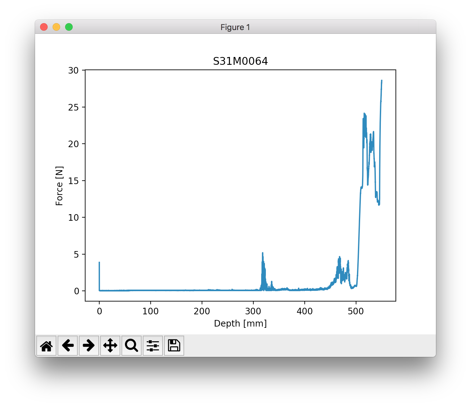
Expore using the tool buttons below the plot! You can even modify the axes and export the plot into an image file.
A Touch of Science
Alright, let’s do some science. In this example, we examine a profile recorded at our Testsite Weissfluhjoch. There’s a crust and a depth hoar layer in this profile. By using command:pyngui, we already identified the layers for you by setting markers. Let’s calculate the mean SSA within the crust and the weight that lies on the depth hoar layer.
from snowmicropyn import Profile
from snowmicropyn import proksch2015

p = Profile.load('profiles/S37M0876.pnt')
p2015 = proksch2015.calc(p.samples)

crust_start = p.marker('crust_start')
crust_end = p.marker('crust_end')

crust = p2015[p2015.distance.between(crust_start, crust_end)]

# Calculate mean SSA within crust
print('Mean SSA within crust: {:.1f} m^2/m^3'.format(crust.P2015_ssa.mean()))

# How much weight lies above the hoar layer?
surface = p.marker('surface')
hoar_start = p.marker('depthhoar_start')
above_hoar = p2015[p2015.distance.between(surface, hoar_start)]
weight_above_hoar = above_hoar.P2015_density.mean() * (hoar_start - surface) / 1000
print('Weight above hoar layer: {:.0f} kg/m^2'.format(weight_above_hoar))
This will print something like:
Mean SSA within crust: 5.5 m^2/m^3
Weight above hoar layer: 98 kg/m^2