API User’s Guide
Data Files
When performing a measurement with SnowMicroPen, the device writes the data
onto its SD card in a binary file with a pnt extension. (Example:
S13M0067.pnt). For each measurment process, a new pnt file is written.
Each pnt file consists of a header with meta information followed by the actual
data, the force samples.
Note
The snowmicropyn package never ever writes into a pnt file. Good to know your precious raw data is always safe.
Corresponding ini files
However, when using functionality of this package, an additional storage to save
other data is required. This storage is an ini file, named like the pnt
file (example from previous section: S13M0067.ini).
First steps
The core class of the API is the snowmicropyn.Profile class. It
represents a profile loaded from a pnt file. By using its static load method,
you can load a profile:
import snowmicropyn
p = snowmicropyn.Profile.load('./S13M0067.pnt')
In the load call, there’s also a check for a corresponding ini file, in this
case for S13M0067.ini.
Logging snowmicropyn’s Version and Git Hash
As a scientist, you may be interested to keep a log so you can reproduce what you calculated with what version of snowmicropyn. The package contains a version string and a git hash identifier.
To access the package’s version string, you do:
import snowmicropyn
v = snowmicropyn.__version__
To access the git hash string of this release, you do:
import snowmicropyn
gh = snowmicropyn.githash()
When exporting data using this module, the created CSV files will also contain a comment as first line with the version string and git hash to identify which version of snowmicropyn was used to create the file.
Warning
However, this is no mechanism to protect a file from later alternation. It’s just some basic information which maybe will be useful to you.
Examples
Some examples will help you get an overview of snowmicropyn’s features.
Hint
To get the code mentioned in this guide, Download the source code of
snowmicropyn. You’ll find the examples in the subfolder examples
and even some pnt files to play around with in the folder
examples/profiles.
Explore properties
In our first example, we load a profile and explore its properties. We set some
markers and finally call the snowmicropyn.Profile.save() so the markers
get saved in an ini file so we don’t lose them.
import logging
import sys

import snowmicropyn

# Enable logging to stdout to see what's going on under the hood
logging.basicConfig(level=logging.DEBUG, stream=sys.stdout)

print(snowmicropyn.__version__)
print(snowmicropyn.githash())

p = snowmicropyn.Profile.load('profiles/S37M0876.pnt')

print('Timestamp: {}'.format(p.timestamp))
print('SMP Serial Number: {}'.format(p.smp_serial))
print('Coordinates: {}'.format(p.coordinates))

p.set_marker('surface', 100)
p.set_marker('ground', 400)
print('Markers: {}'.format(p.markers))

# We don't want to lose our markers. Call save to write it to an ini
# file named like the pnt file.
p.save()
Batch exporting
You’re just home from backcountry where you recorded a series of profiles with your SnowMicroPen and now want to read this data with your tool of choice which supports reading CSV files? Then this example is for you!
import glob

from snowmicropyn import Profile

match = 'profiles/*.pnt'

for f in glob.glob(match):
    print('Processing file ' + f)
    p = Profile.load(f)
    p.export_samples()
    p.export_meta(include_pnt_header=True)
    p.export_derivatives()
After you executed this example, there will be a ..._samples.csv and a
..._meta.csv for each pnt file in the directory.
Plotting
In this example, we use the delightful matplotlib to explore the penetration signal of a profile.
from matplotlib import pyplot as plt

from snowmicropyn import Profile

p = Profile.load('profiles/S37M0876.pnt')

# Plot distance on x and samples on y axis
plt.plot(p.samples.distance, p.samples.force)

# Prettify our plot a bit
plt.title(p.name)
plt.ylabel('Force [N]')
plt.xlabel('Depth [mm]')

# Show interactive plot with zoom, export and other features
plt.show()
When this code is executed, a window like the following should open:
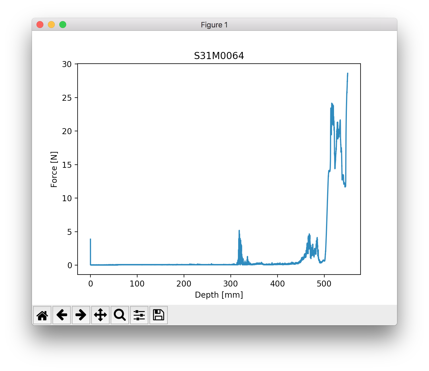
Explore using the tool buttons below the plot! You can even modify the axes and export the plot into an image file.
A Touch of Science
Alright, let’s do some science. In this example, we examine a profile recorded at our test site Weissfluhjoch. There’s a crust and a depth hoar layer in this profile. By using pyngui, we already identified the layers for you by setting markers. Let’s calculate the mean specific surface area (SSA) within the crust and the weight that lies on the depth hoar layer.
from snowmicropyn import Profile
from snowmicropyn import proksch2015

p = Profile.load('profiles/S37M0876.pnt')
p2015 = proksch2015.calc(p.samples)

crust_start = p.marker('crust_start')
crust_end = p.marker('crust_end')

crust = p2015[p2015.distance.between(crust_start, crust_end)]

# Calculate mean SSA within crust
print('Mean SSA within crust: {:.1f} m^2/m^3'.format(crust.P2015_ssa.mean()))

# How much weight lies above the hoar layer?
surface = p.marker('surface')
hoar_start = p.marker('depthhoar_start')
above_hoar = p2015[p2015.distance.between(surface, hoar_start)]
weight_above_hoar = above_hoar.P2015_density.mean() * (hoar_start - surface) / 1000
print('Weight above hoar layer: {:.0f} kg/m^2'.format(weight_above_hoar))
This will print something like:
Mean SSA within crust: 5.5 m^2/m^3
Weight above hoar layer: 98 kg/m^2
Using Different Parameterizations
Depending on your SMP device and/or your climatic settings different parameterizations to derive observables from the raw SMP measurements may be preferable. Have a look at the Parameterizations help topic for details on what’s available.
In the GUI you are able to select them individually, and programmatically this is done by giving their short names.
The names are found in the shortname property in the respective
implementations (in the parameterizations subdirectory) and can
be e. g. “P2015”, “CR2020”, “K2020a” or “K2020b”.
"""Showcase for how to programmatically use different
parameterizations."""

import os
import snowmicropyn as smp

EX_PATH = '../examples/profiles/S37M0876'

pro = smp.Profile.load('../examples/profiles/S37M0876.pnt')
# Output with default Proksch 2015 parameterization:
pro.export_derivatives()
os.rename(EX_PATH + '_derivatives.csv', EX_PATH + '_derivatives_P2015.csv')

# Switch to Calonne/Richter parameterization:
pro.export_derivatives(parameterization='CR2020')
os.rename(EX_PATH + '_derivatives.csv', EX_PATH + '_derivatives_CR2020.csv')

# Now with King 2020b, but as an experiment we change
# a few properties before calculation, namely the size of the
# moving window and the overlap factor:
smp.params['K2020b'].window_size = 2.5
smp.params['K2020b'].overlap = 70
pro.export_derivatives(parameterization='K2020b')
os.rename(EX_PATH + '_derivatives.csv', EX_PATH + '_derivatives_K2020x.csv')
Working with the Machine Learning Module
Have a look at how snowmicropyn uses machine learning for its grain shape estimation. To reiterate, this is done in order to be able to provide valid snowpit CAAML output. For example, niViz needs the grain shape to display something.
In order to accomplish this, snowmicropyn offers a machine learning interface which will try to learn the connection between the measured SMP microparameters and known grain shapes.
As usual you can control this interface through the API and via the GUI. Have a look at the shipped ai example program to see how to control the API. The GUI on the other hand is opened when exporting to CAAML.
Snowmicropyn ships a training data file which has been pre-computed for your convenience, so ideally when enabling grain shape export it should produce valid output. However, it will be trained with a limited amount of profiles from a certain climate setting so if available you should produce your own training data.
To do so you need to specify a folder containing SMP data and grain shape information, as well as the method used for parsing. For example, method ‘exact’ expects a folder that contains both pnt files and caaml files (same base name) where the grain shape is taken from the caaml file at measurement depth. Method ‘markers’ on the other hand expects pnt files only but they must have markers set for the grain types.
The folder tools contains a script to download and prepare both of
these types of datasets, in this case from the RHOSSA campaign (follow the
links therein for more information about this dataset, and about the
markers’ naming conventions).
Obviously if you are inherently interested in the grain shape then these methods have their limits - again, the provided example performs some test scores to give an idea about the accuracy.